Arix Technologies sought to evaluate the MRUT SIZING application using VOLTA 2 for their inspection operations. To assess the application's performance, they provided a pipe sample containing conditions commonly encountered in the field, along with four artificial defects designed to challenge remaining wall thickness estimation. The Arix team aimed to confirm that Innerspec’s solution could accurately detect and differentiate all four defects while providing a reliable estimate of the remaining wall.
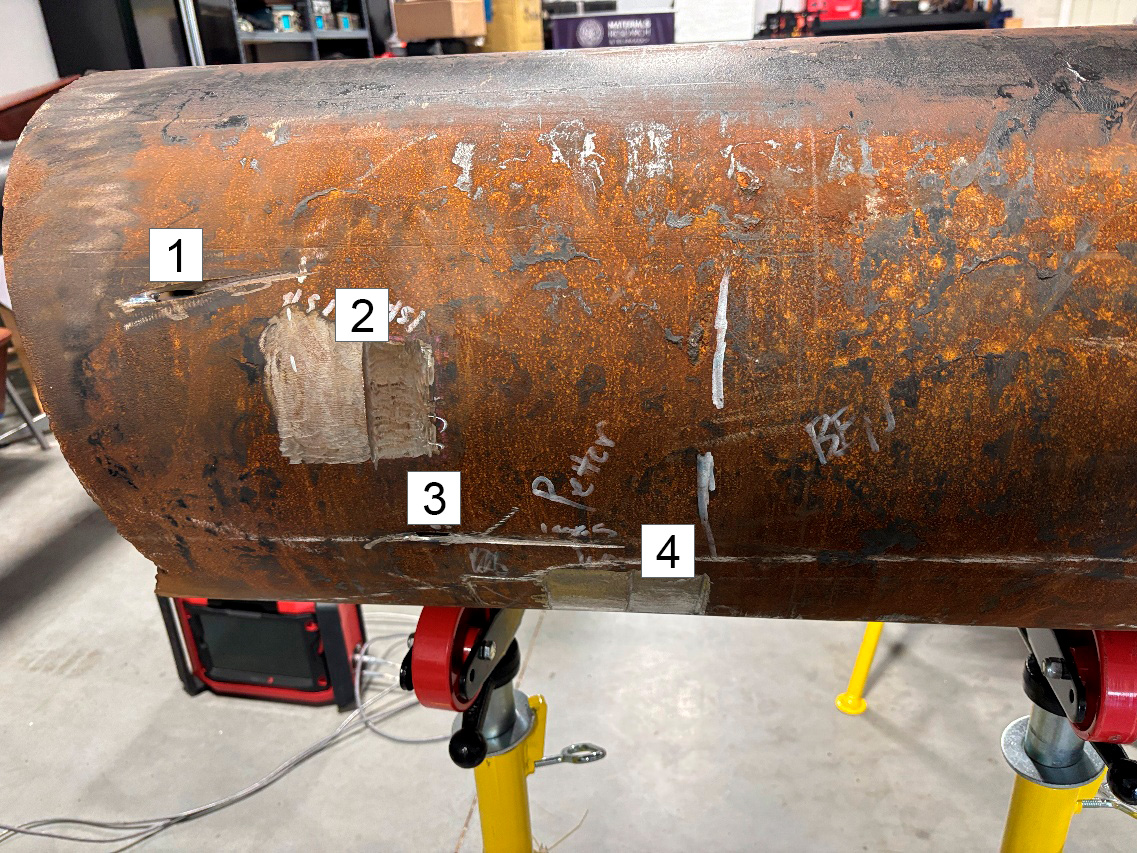
The sample was a 16-inch OD carbon steel pipe with a 0.250-inch WT and four artificial defects. These defects overlapped both axially and circumferentially, presenting an additional challenge for estimating the remaining wall thickness. The four defects, as shown in Figure1, consisted of:
The sample presented general ID corrosion along the full part. This corrosion impeded the propagation of the SH1 (dispersive) mode used for the cutoff-frequency technique. The team hadn’t been able to inspect this sample with an instrument that used only the cutoff-frequency technique.
The equipment used for these tests is Innerspec VOLTA 2, a high-power, two-channel portable ultrasonic instrument designed for use with Electro Magnetic Acoustic Transducers (EMATs). It incorporates a proprietary pulser architecture capable of generating tone bursts from 1 to 10 cycles with output amplitudes up to 1,000 Vpp. The pulser design supports the high excitation energy requirements typical of EMAT-based inspections while maintaining a compact, field-deployable form factor.
VOLTA can be used to perform any EMAT technique, including Thickness Measurement, Weld Inspection, as well as Medium Range and Long-Range Guided Wave techniques.

The technique used for this application permits inspecting hidden areas of the circumference of a pipe by scanning axially along the pipe. It is especially well-suited for the detection and sizing of Corrosion Under Pipe Supports (CUPS). The MRUT SIZING scanner generates guided waves via a magnetostrictive (MS) strip adhered axially on the pipe.
The technique combines amplitude-based (SH0 wave mode) and frequency-based (SH1 wave mode) measurement techniques to provide highly accurate remaining wall thickness (RWT) measurements along the pipe. This defect sizing technique is designed to be used on pipes 0.25” to 1” in thickness (6-25 mm) and diameters ranging from NPS 6 to NPS 24.
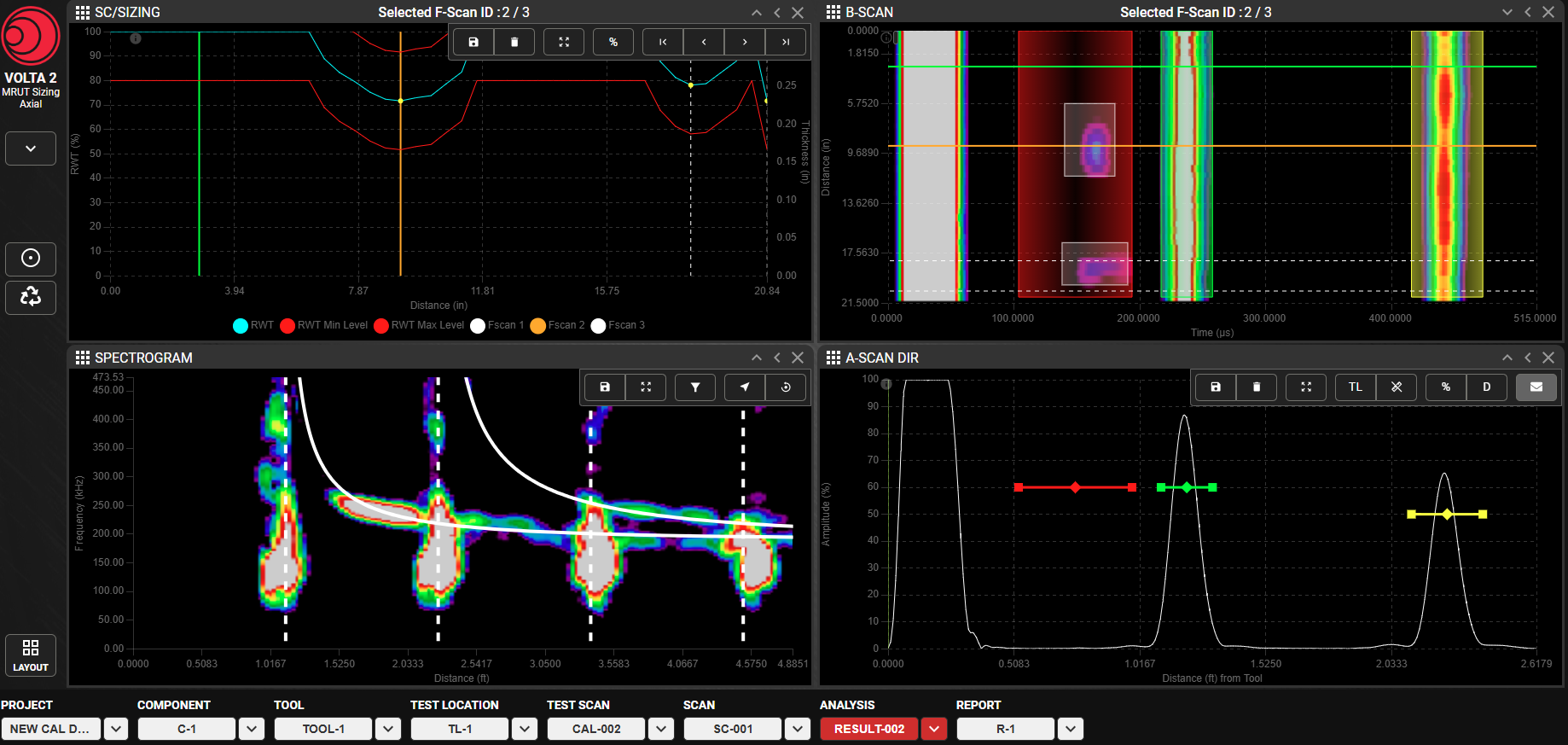
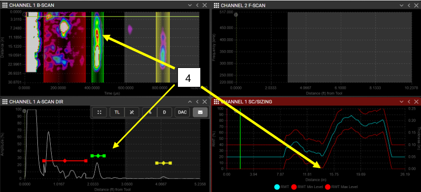
Following data acquisition in SCAN, the software integrates amplitude and frequency sizing during the ANALYSIS step. At the discrete points where frequency scans were captured, automatic cutoff measurements are combined with amplitude data. The resulting integrated measurements are then displayed in the SC/Sizing chart, providing enhanced accuracy for the remaining wall thickness profile.
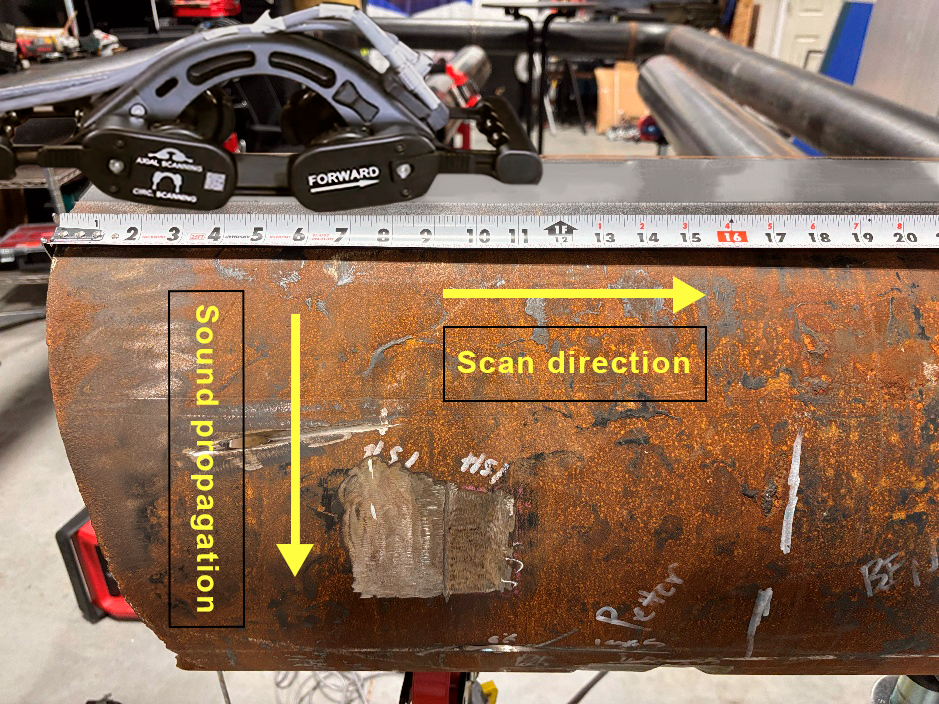
For this scan, the strip was positioned 180 mm (7”) from the defective area. The strip should be positioned beyond the suspected defect zone to establish a baseline signal in a clean area of the pipe.
Once the strip is adhered to the pipe, the baseline must be established for both channels (Channel 1 – Amplitude, Channel 2 – Frequency) in a nominal section of the pipe. It is important to note that "defect-free" or "clean" are relative terms and do not imply the pipe is in pristine condition; rather, they indicate that the area is in good condition relative to the area of interest.
The calibration results for Channel 1 (Amplitude) and Channel 2 (Frequency) are shown in the following two figures:
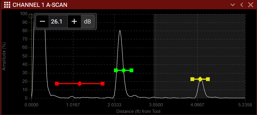
Channel 1 (amplitude), using SH0 wave mode, was able to identify an area where the wrap-around signals were strong, and reflections were at their lowest. The calibration process sets the gain so that the first wrap-around signal reaches 80% screen height. In this case, the calculated gain—which will serve as the baseline for the subsequent inspection scan—was set to 26.1 dB.
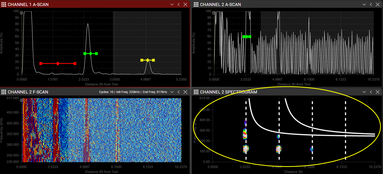
At the same 'clean' location, it was observed that the Channel 2 calibration (frequency sweep) had a negligible or non-existent response. Additionally, the baseline of the signal around the pipe was rough, resulting in a grainy B-Scan. This lack of frequency signal indicates that the SH1 wave mode cannot propagate around the pipe, which is a strong sign of internal corrosion. This is a known limitation of the frequency-cutoff technique, which relies on the dispersive SH1 mode to calculate the remaining wall thickness.
During the scan, the generalized corrosion was further corroborated by the amplitude B-scan, which was also grainy due to small reflections throughout the pipe. Due to this condition, the remaining wall assessment was performed entirely using the amplitude technique (SH0).
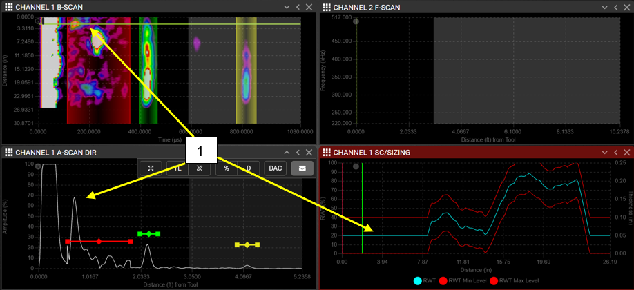
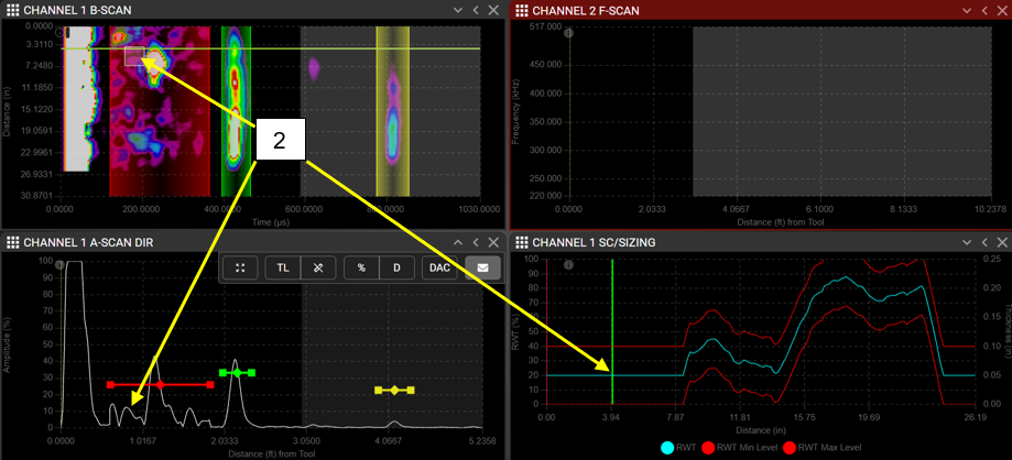
The amplitude channel, utilizing the SH0 mode, was able to generate strong signals. This technique accounts for both direct reflections from defects and wrap-around attenuation.
The calibration process revealed general ID corrosion across the entire sample. This corrosion impeded the propagation of the SH1 (dispersive) mode used for the cutoff-frequency technique, a finding corroborated by the grainy B-scan in the amplitude channel. This condition explains why the sample could not be inspected using an instrument that relies solely on the cutoff-frequency technique.
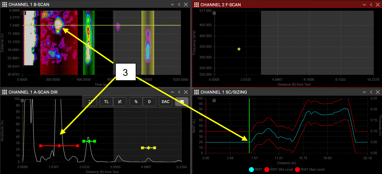
The defects overlapped both axially and circumferentially, posing an additional challenge for estimating the remaining wall thickness. Despite these difficult material conditions and complex defect geometries, the VOLTA 2, with MRUT SIZING AXIAL, successfully detected and differentiated all four defects while providing a reliable estimate of the remaining wall.